COVID-19 Data Modelling
This the modelling assignment. The thing that will be modeled is the COVID-19 growth in Indonesia. Hence, the date in the future can be predicted during the pandemic by utilizing the basic model which is found through this assignment.
The data is based on the following URL:
| https://www.ecdc.europa.eu/en/publications-data/download-todays-data-geographic-distribution-covid-19-cases-worldwide |
The country which is chosen to do the modelling is Indonesia. Such data contains about 101 rows. However, as the existing cases starts from 3/2/2020, the number of rows which is used to do the modelling is only 37 rows.
Data Exploration
while exploring the data, I found there is the non-sequence data. Therefore, I sort the data based on the sequence date in order to obtain the better growth. The following code is the data exploration code for Indonesia case.
#read directory

os.chdir('D:/George Mason University/Semester 2/Analytics Big Data to Information/Assignment 8')
os.getcwd()


#Import the data1
data1 = pd.read_csv('COVID-19-geographic-disbtribution-worldwide-2020-04-16.csv', sep = ',')
data1
data1.head(10)
data1.info()
data1['countriesAndTerritories']

#setdata1 Indonesia
data1_indonesia = data1.query('countriesAndTerritories == "Indonesia"')
len(data1_indonesia.index)
data1_indonesia2 = data1_indonesia.sort_values(by='dateRep')
data1_indonesia2.info()
data1_indonesia3 = data1_indonesia2[['dateRep', 'day', 'month', 'year', 'cases', 'deaths', 'popData2018', 'countriesAndTerritories']]
data1_indonesia3.head(50)

#convert to array for sorting
dateRep1 = np.array(data1_indonesia3['dateRep'])
day1 = np.array(data1_indonesia3['day'])
month1 = np.array(data1_indonesia3['month'])
year1 = np.array(data1_indonesia3['year'])
cases1 = np.array(data1_indonesia3['cases'])
deaths1 = np.array(data1_indonesia3['deaths'])
popData1 = np.array(data1_indonesia3['popData2018'])
countriesAndTerritories1 = np.array(data1_indonesia3['countriesAndTerritories'])

###############################################################################
#sort based on year
###############################################################################
i = 0
while (i < (len(data1_indonesia3) - 1)):
    j = 0
    while (j < (len(data1_indonesia3)-i-1)):
        if (year1[j] > year1[j + 1]):
            temp1 = year1[j]
            year1[j] = year1[j + 1]
            year1[j + 1] = temp1
            temp2 = day1[j]
            day1[j] = day1[j + 1]
            day1[j + 1] = temp2
            temp3 = month1[j]
            month1[j] = month1[j + 1]
            month1[j + 1] = temp3
            temp4 = cases1[j]
            cases1[j] = cases1[j + 1]
            cases1[j + 1] = temp4
            temp5 = deaths1[j]
            deaths1[j] = deaths1[j + 1]
            deaths1[j + 1] = temp5
            temp6 = dateRep1[j]
            dateRep1[j] = dateRep1[j + 1]
            dateRep1[j + 1] = temp6
            temp7 = popData1[j]
            popData1[j] = popData1[j + 1]
            popData1[j + 1] = temp7

        j = j + 1
    i = i + 1

###############################################################################
#sort based on month
###############################################################################

i = 0
while (i < (len(data1_indonesia3) - 1)):
    if (year1[i] == year1[i + 1]):
        print("same year")

        j = i;
        while (j < (len(data1_indonesia3) - 1)):
            k = j
            while (k < (len(data1_indonesia3)-i-1)):
                print('sorting process')
                if (month1[k] > month1[k + 1]):
                    temp1 = year1[k]
                    year1[k] = year1[k + 1]
                    year1[k + 1] = temp1

                    temp2 = day1[k]
                    day1[k] = day1[k + 1]
                    day1[k + 1] = temp2

                    temp3 = month1[k]
                    month1[k] = month1[k + 1]
                    month1[k + 1] = temp3

                    temp4 = cases1[k]
                    cases1[k] = cases1[k + 1]
                    cases1[k + 1] = temp4

                    temp5 = deaths1[k]
                    deaths1[k] = deaths1[k + 1]
                    deaths1[k + 1] = temp5

                    temp6 = dateRep1[k]
                    dateRep1[k] = dateRep1[k + 1]
                    dateRep1[k + 1] = temp6

                    temp7 = popData1[k]
                    popData1[k] = popData1[k + 1]
                    popData1[k + 1] = temp7
                k = k + 1
            j = j + 1
    else:
        print("different year")
    i = i + 1
###############################################################################
#sort based on day
###############################################################################

i = 0
while (i < (len(data1_indonesia3) - 1)):
    if (year1[i] == year1[i + 1]):
        print("same year")

        j = i;
        while (j < (len(data1_indonesia3) - 1)):
            k = j
            while (k < (len(data1_indonesia3)-i-1)):

                if (month1[k] == month1[k + 1]):
                    print("same month")

                    l = k
                    while ((l < (len(data1_indonesia3)-i)) and (month1[l] == month1[l + 1])):
                        if (day1[l] > day1[l + 1]):
                            temp1 = year1[l]
                            year1[l] = year1[l + 1]
                            year1[l + 1] = temp1

                            temp2 = day1[l]
                            day1[l] = day1[l + 1]
                            day1[l + 1] = temp2

                            temp3 = month1[l]
                            month1[l] = month1[l + 1]
                            month1[l + 1] = temp3

                            temp4 = cases1[l]
                            cases1[l] = cases1[l + 1]
                            cases1[l + 1] = temp4

                            temp5 = deaths1[l]
                            deaths1[l] = deaths1[l + 1]
                            deaths1[l + 1] = temp5

                            temp6 = dateRep1[l]
                            dateRep1[l] = dateRep1[l + 1]
                            dateRep1[l + 1] = temp6

                            temp7 = popData1[l]
                            popData1[l] = popData1[l + 1]
                            popData1[l + 1] = temp7

                        l = l + 1

                else:
                    print("different month")
                k = k + 1
            j = j + 1
    else:
        print("different year")
    i = i + 1
###############################################################################
#New Data Frame for setdata1 Indonesia
###############################################################################
data1_indonesia4 = pd.DataFrame({'dateRep' : dateRep1,
                                 'day' : day1,
                                 'month' : month1,
                                 'year' : year1,
                                 'cases' : cases1,
                                 'deaths' : deaths1,
                                 'popData2018' : popData1,
                                 'countriesAndTerritories' : countriesAndTerritories1})

data1_indonesia4 = data1_indonesia4.query('cases > 0').reset_index(drop=False).reset_index(drop=False)

#data1_indonesia4 = data1_indonesia4[['level_0', 'dateRep', 'day', 'month', 'year', 'cases', 'deaths', 'popData2018']]

data1_indonesia4 = data1_indonesia4[['level_0', 'dateRep', 'day', 'month', 'year', 'cases']]

#data1_indonesia4.columns = ['Timestep', 'dateRep', 'day', 'month', 'year', 'cases', 'deaths', 'popData2018']

data1_indonesia4.columns = ['Timestep', 'dateRep', 'day', 'month', 'year', 'cases']

data1_indonesia4.head(16)
|
create a basic model of the growth of the virus in that country
prior to decide the best basic model, the summary of the model should be performed at first in order to check the R-Square value. In this case, since the R-Square value has the best value which almost approach to 1, and already been proved by analyzing the diagnostic plot, so the model seems to be the best basic model. The model summary is shown by the following summary:
                            OLS Regression Results
==============================================================================
Dep. Variable:                  cases   R-squared:                       0.857
Model:                            OLS   Adj. R-squared:                  0.853
Method:                 Least Squares   F-statistic:                     215.0
Date:                Sun, 19 Apr 2020   Prob (F-statistic):           9.38e-17
Time:                        00:21:18   Log-Likelihood:                -194.53
No. Observations:                  38   AIC:                             393.1
Df Residuals:                      36   BIC:                             396.3
Df Model:                           1
Covariance Type:            nonrobust

==============================================================================
                 coef    std err          t      P>|t|      [0.025      0.975]
------------------------------------------------------------------------------
const        -31.6437     13.224     -2.393      0.022     -58.464      -4.823
Timestep       9.0163      0.615     14.662      0.000       7.769      10.263
==============================================================================
Omnibus:                        7.199   Durbin-Watson:                   1.538
Prob(Omnibus):                  0.027   Jarque-Bera (JB):                6.598
Skew:                           0.645   Prob(JB):                       0.0369
Kurtosis:                       4.582   Cond. No.                         42.2
============================================================================== |
The following code is used to perform the summary above:
X = data1_indonesia4.Timestep X = sm.add_constant(X) y1 = data1_indonesia4.cases model1 = sm.OLS(y1, X) model_fit1 = model1.fit() print(model_fit1.summary()) |
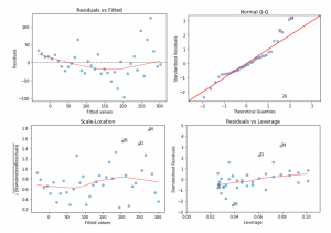
The diagnostic plot is performed while analyzing the model. The diagnostic plot is shown through the following picture.

According to the four diagnotic plot above, it can be concluded that the basic model is the best fit for the data. The first plot, which is the Residuals vs Fitted, shows that the model does not violate the linear assumtions since the red line still adjacent to the dash line. Also, the spread residuals still surrounds the red line without many distinct patterns of the red line.
The second plot shows a little violations to the normality assumptions since there are some residuals with the extreme values than would be expected. However, even though the extreme data are omited, that would not make a lot of change since all the data are beyond the cook’s distance as shown through plot number 4, the residuals vs leverage.
The third plot shows that the red line does not perfectly appear to be horizontal. However, as long as the red line is not the same as y = 0, it does not violate the equal variance.
The basic model of the residuals is y = (-31.6437) + 9.0163X. The declaration code of such model is shown through the following:
#basic model function = #y = (-31.6437) + 9.0163X def linear_predictions(t): return (-31.6437) + (9.0163 * t) |
The actual data and the predicted data shown by the following:
Timestep dateRep day month year cases PredictedCases 0 0 3/2/2020 2 3 2020 2 -31.6437 1 1 3/7/2020 7 3 2020 2 -22.6274 2 2 3/9/2020 9 3 2020 2 -13.6111 3 3 3/11/2020 11 3 2020 13 -4.5948 4 4 3/12/2020 12 3 2020 15 4.4215 5 5 3/14/2020 14 3 2020 35 13.4378 6 6 3/15/2020 15 3 2020 27 22.4541 7 7 3/16/2020 16 3 2020 21 31.4704 8 8 3/17/2020 17 3 2020 17 40.4867 9 9 3/18/2020 18 3 2020 38 49.5030 10 10 3/20/2020 20 3 2020 55 58.5193 11 11 3/21/2020 21 3 2020 82 67.5356 12 12 3/22/2020 22 3 2020 141 76.5519 13 13 3/23/2020 23 3 2020 64 85.5682 14 14 3/24/2020 24 3 2020 65 94.5845 15 15 3/25/2020 25 3 2020 107 103.6008 16 16 3/26/2020 26 3 2020 104 112.6171 17 17 3/27/2020 27 3 2020 103 121.6334 18 18 3/28/2020 28 3 2020 153 130.6497 19 19 3/29/2020 29 3 2020 109 139.6660 20 20 3/30/2020 30 3 2020 130 148.6823 21 21 3/31/2020 31 3 2020 129 157.6986 22 22 4/1/2020 1 4 2020 114 166.7149 23 23 4/2/2020 2 4 2020 149 175.7312 24 24 4/3/2020 3 4 2020 113 184.7475 25 25 4/4/2020 4 4 2020 196 193.7638 26 26 4/5/2020 5 4 2020 106 202.7801 27 27 4/6/2020 6 4 2020 181 211.7964 28 28 4/7/2020 7 4 2020 218 220.8127 29 29 4/8/2020 8 4 2020 247 229.8290 30 30 4/9/2020 9 4 2020 218 238.8453 31 31 4/10/2020 10 4 2020 337 247.8616 32 32 4/11/2020 11 4 2020 219 256.8779 33 33 4/12/2020 12 4 2020 330 265.8942 34 34 4/13/2020 13 4 2020 399 274.9105 35 35 4/14/2020 14 4 2020 316 283.9268 36 36 4/15/2020 15 4 2020 282 292.9431 37 37 4/16/2020 16 4 2020 297 301.9594 |
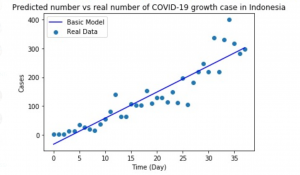
Other than that, the illustration of the basic model is such the follow:

The potential limitations of the model are the extreme spike of the data can’t be predicted. Other than that, as shown in the second plot of the diagnostic plot, the data model does not perfectly match the residuals since the head and the tail does not perfectly match the diagonal line.
